Arweave 2.6
Arweave is a permanent data storage network. This document describes version 2.6, an upgrade to the network that achieves the following objectives:
- Lowers the storage acquisition cost for the network by encouraging miners to use cheaper drives to store data, rather than optimizing for drive speed.
- Lessens energy wastage in the network by directing a greater proportion of mining expenditure to the useful storage of data.
- Incentivizes miners to self-organize into full replicas of the Arweave dataset, allowing for faster routing to data and an even more 'flat' distribution of data replication.
- Allows for better dynamic price
Per GB/Hourstorage cost estimation in the network.
Mechanism
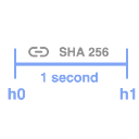
- A SHA-256 hash chain produces a mining hash once every second
- Miners select an index of a partition they store to begin mining
- A recall range is generated in the miners partition and another at a random weave location
- Chunks in the first recall range are checked as a potential block solutions
- The second range may also be checked but solutions there require a hash from the first.
| Mining Element | Description |
|---|---|
| Sometimes referred to as "the weave", Arweave data is divided into a uniform collection of chunks that can be evenly spread across the Arweave network. Additionally, this storage model enables a common addressing scheme used to identify chunks anywhere in the weave. | |
 Chunk Chunk |
Chunks are contiguous blocks data, typically 256KB in length. The packing and hashing of these chunks is how miners win the right to produce new blocks and prove they are storing replicas of the data during the SPoRA mining process. |
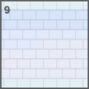 Partition Partition |
Partitions are new in 2.6 and describe a logical addressing scheme layered over top of the weave at 3.6TB intervals. Partitions are indexed from 0 at the beginning of the weave up to however many partitions required to span the entirety of the weave (up to the block seeding the hash chain). |
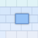
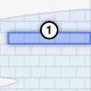 Recall range Recall range |
A recall range is a continuous range of chunks beginning at a specific offset in the weave and extending 100MiB in length. |
 Potential solutions Potential solutions |
Each 256KiB offset in a recall range contains a potential solution to the mining puzzle. As part of the mining process each solution candidate is hashed to test if it meets the difficulty requirements of the network. If it does, the miner wins the right to produce a new block and earn mining rewards. If not, the miner continues on to mine the next 256KiB interval in the recall range. |
 Hash Chain Hash Chain |
Hash chains result from the successive application of a cryptographic hashing function (SHA-256 in this case) to a piece of data. Because the process cannot be parallelized (and consumer grade CPUs already have optimized SHA-256 circuits) hash chains verify a delay has occurred by requiring a certain number of successive hashes between operations. |
 Mining Hash Mining Hash |
After a sufficient number of successive hashes (to create a 1 second delay) the hash chain produces a hash which is considered valid for mining. It's worth noting that mining hashes are consistent across all miners and verifiable by all miners. |
Optimal Mining Strategy
Packing unique replicas
Arweave seeks to maximize the number of replicas stored on the network. To that end it must make the chances of winning the mining competition depend mainly on the number of stored replicas per miner.
Winning solutions to the mining game require that the recall chunk be packed in a specific format. Packing involves providing a packing key to RandomX and having it generate a 2MiB scratchpad of entropy over multiple iterations. The first 256KiB of the scratchpad are then used to encrypt the chunk. Unpacking works the same way, provide the packing key, generate the scratchpad and use the first 256KiB to decrypt/reveal the original chunk.
In version 2.5 the packing key was the SHA256 hash of the concatenation of the chunk_offset and tx_root. This ensured every mining solution came from a unique replica of a chunk in a specific block. If multiple copies of a chunk existed at different locations in the weave, each one would need to be packed individually to be a solution candidate.
In version 2.6 this packing key is extended to be the SHA256 hash of the concatenation of chunk_offset, tx_root, and miner_address. This means that each replica is also unique per mining address.
Data Distribution
The mining algorithm has to incentivize miners to construct complete replicas that result in a uniform data distribution across the network. There has to be a strong preference for a single entire replica over a partial one duplicated several times.
One strategy a miner might pursue is to store multiple copies of a partial data set.
Following this strategy, the miner syncs the first 4 partitions of the weave and instead of filling available space with unique partitions; they replicate the same 4 partitions each packed with a unique mining address.
Each time a mining hash is produced, the miner is able to use it to target each partition on the disk for the first recall range. Infrequently, but occasionally the second recall range will fall in a partition they store and they will be able to mine it as well. This guarantees them ~400 potential solutions per partition per second.
A more optimal strategy given the two recall range mechanism is to store as many unique partitions as possible. The following diagram illustrates using a single mining address with 16 partitions as opposed 4 partitions replicated multiple times each with it's own mining address.
By adopting this strategy the miner greatly increases the chances of having the second recall range fall in a partition they store. More often than not leading to two recall ranges per partition. If the miner stores all partitions they can guarantee 800 potential solutions per partition.
This creates a significant advantage for miners choosing to store a complete replica over multiple copies of partial replicas.
Capping Drive Speed Incentives
Because recall ranges are contiguous blocks of memory, they minimize the amount of read head movement on Hard Disk Drives (HDDs). This optimization brings the read performance of HDDs in line with the more expensive Solid State Drives (SSDs) but at a lower cost.
One consequence of this two part recall range mechanism is that the drive speed to drive space ratio for mining can now be calculated. The result is a balanced mining process where any increase in earnings from faster drives would not offset the expense of purchasing and operating those drives.
A miner could choose expensive SSDs capable of transferring four recall ranges per partition per second. This would give them a slight speed advantage in evaluating potential solutions but it wouldn't provide any additional solutions per second over a miner using cheaper HDDs. Faster drives are more expensive and any time spent idle squanders the utility of that speed at the miners expense.
Energy Efficiency
To minimize the energy mining consumes and ensure energy expenditures are spent verifying storage of complete replicas the mining algorithm must create diminishing returns for other energy intensive mining strategies.
An example of an alternative mining strategy would be to try to take advantage of compute resources instead of storage.
Why would a miner do this? Many reasons, an entirely plausible scenario is that the miner has already made a considerable investment in compute hardware (perhaps for mining another proof of work blockchain) and is looking for ways to maximize the return on that investment.
The miner would prefer to avoid the cost of storing an entire replica of the weave. Even if they did purchase the hardware required to do so, the two recall range per partition cap could leave most of their compute resources idle. To fully utilize their compute they'd have to store multiple replicas and incur the additional storage costs associated with doing so. A capital cost the miner would prefer to avoid if at all possible.
How would a miner go about winning the mining competition without paying for storage?
They would need access to a unlimited source of hashes that they could use to keep all of their compute resources grinding on a single storage partition. How could they do this when the hash chain only produces a valid mining hash once a second?
Instead of relying on storing as many partitions as possible to maximize potential solutions, the miner would instead generate as many mining addresses as needed to saturate their compute. But how would this be viable? Potential solutions need to be packed with the miner_address to be considered valid. Wouldn't this require storing a copy of the partition packed for each mining address thus incurring additional storage costs anyway? What if instead the miner stored the partition as raw unpacked chunks. Then when evaluating the recall range for each mining address the miner could use their compute resources to pack the chunks on demand.
Let's say storing a full replica and following the two recall range per partition cap produced 100k potential solutions per second. If a compute centric miner was able to test 100k+ potential solutions (bounded only by the amount of compute available) grinding mining addresses, they could gain an advantage in the mining competition. If profitable, this could become the dominant mining strategy negatively impacting data replication and undermining Arweaves utility as a protocol for permanent storage.
Capping Compute Incentives
The key to discouraging grinding mining addresses is to ensure the cost (in time and energy) required to pack a chunk solution on demand for a mining address is far greater than storing prepacked chunks for the same address.
To ensure that packing on demand is both time consuming and energy intensive, the packing function includes a PACKING_DIFFICULTY parameter. This parameter specifies the number of rounds of RandomX required to generate a valid scratchpad to be used as entropy for the packing cypher.
A balance must be struck between the making the speed at which new chunks can be packed fast enough that the write throughput of the network is not impared and difficult enough that packing on demand is significantly less efficient than reading prepacked chunks from disk.
Version 2.6 sets the PACKING_DIFFICULTY at 45*8 RandomX programs per chunk which takes about as much time as 30 standard RandomX hashes. This strikes a reasonable balance between limiting the speed of on-demand packing and the volume of data a miner can pack in a day.
Even if packing on demand is slower for one CPU, if the energy cost of packing on demand across many CPU's is similar to that of operating drives full of pre-packed replicas it might still be profitable to grind mining addresses.
We have made a calculator exploring the trade-offs, suggesting the choices for the protocol parameters (recall range size, partition size, PACKING_DIFFICULTY, etc.) to make packing complete replicas the most economically viable strategy.
Link to calculator page (Source)
The calculator computes the cost of operating on demand packing as being 19.86 times more expensive than operating prepacked replicas (Labeled as "On-Demand Cost / Honest Cost" in the calculator).
Dynamic Pricing
At its core the price of storage on Arweave is determined by the price to store 1GB of data for one hour or PGBH as expressed by the following equation.
Where HDDprice is the market price of a hard drive on the network, HDDsize is the capacity of the drive in GB, and HDDMTBF is the mean time between failures for hard drives.
Difficulty based dynamic pricing was reintroduced with version 2.5 with the price adjusting once every 50 blocks within a bound of +/- 0.5%.
What was difficult calculate in version 2.5 was the speed of drives in use by miners. Because faster drives are more expensive than slower drives the HDDprice required estimation of the average drive speed for the network. In version 2.6 the protocol describes a maximum incentivized drive speed which forms the basis of HDDprice in calculations.
Drives will need to produce two recall ranges worth of potential solutions per partition per second. With each recall range being 100MiB, we can state that a drive must have bandwidth capable of transferring 200MiB per stored 3.6TB partition per second. Any drive performance in excess of this target bandwidth is a wasted expense that negatively affects the miners profitability. Deploying drives with less than the required bandwidth means the miner will also be less profitable as they will not be competitive. This provides a solid basis for calculating HDDprice and eliminates the dependence on an average drive speed for price calculations.
From here we can examine the difficulty of the network to determine the hash rate and from that calculate the number of partitions stored. This is possible because at peak utilization partitions will produce 800 hashes per second (the amount of potential solutions provided by two recall ranges). We can look at the per second hash rate of the network and calculate the number of partitions that must be stored to produce that number of hashes. Because the protocol incentivizes storing unique partitions we can divide (partition_count * 3.6TB) by weave_size and calculate an approximate number of replicas.
In order to offer reliable service the protocol must charge a price sufficient to fund a target number of replicas such that in the event of catastrophic failures it is highly probable that at least one replica survives long enough for new copies to be made.
We conducted research on the mean time between failures for modern drives and have concluded that a target of 15 replicas is a conservative minimum to ensure the long term data persistence on Arweave. For details of how we arrived at these conclusions, please review our approach here.
These factors form the basis of calculating the minimum fee required to fund sufficient replication of data on the network to ensure its long term survival.
Hash Chain Validation
Part of accepting new blocks is validating that they were formed correctly. If the validator is in sync with the block producer they will be able to validate the new blocks mining hash from their own recently produced mining hashes.
In the case that the validator is not at the current head of the hash chain, each block includes 25 40ms checkpoints. Each of these checkpoints are the result of successively hashing for 40ms and when assembled represent a one second interval from the previous blocks mining hash.
Before a validator gossips a newly received block to its peers it quickly validates the first 25 checkpoints in parallel. If the 40ms checkpoints are validated the block is gossiped and the complete sequence of checkpoints is validated.
Complete checkpoint validation is accomplished by hashing the remaining checkpoints in parallel. The first 25 checkpoints are followed by 500 one second checkpoints, then 500 two second checkpoints, with the checkpoint spacing doubling for every subsequent set of 500 checkpoints.
Producing new mining hashes at the head of the hash chain must be done sequentially but the checkpoints generated during this process can be verified in parallel. This allows themining hash for a block to be validated in much less time than it took to create the hash chain that generated it.
Seeding the hash chain
In the case where a miner or mining pool has a slightly faster implementation of SHA 256, it may be possible for their hash chain to run ahead of the rest of the network. Over time that small speed advantage may accumulate into a significant amount of hash chain drift, making the mining hashes it produces out of sync with the rest of the validators. This could result in number of undesirable fork and reorg scenarios.
To reduce the potential for hash-chain drift, Arweave synchronizes the global hash chain with entropy from a historical block on a fixed interval. This provides a new seed for the hash chain every so often with the effect of syncronizing the individual miners hash-chains on a well known and confirmed block.
The hash chain interval is anchored to the hash chain with a new seed block being chosen every 50 * 120 mining hashes. This places the seed blocks approximately ~50 Arweave blocks apart but as there is some variance in blocktimes the seed block may appear sooner or later than 50 blocks.